THE ENVIRONMENTS – BI SIZING & HARDWARE (Staging) –
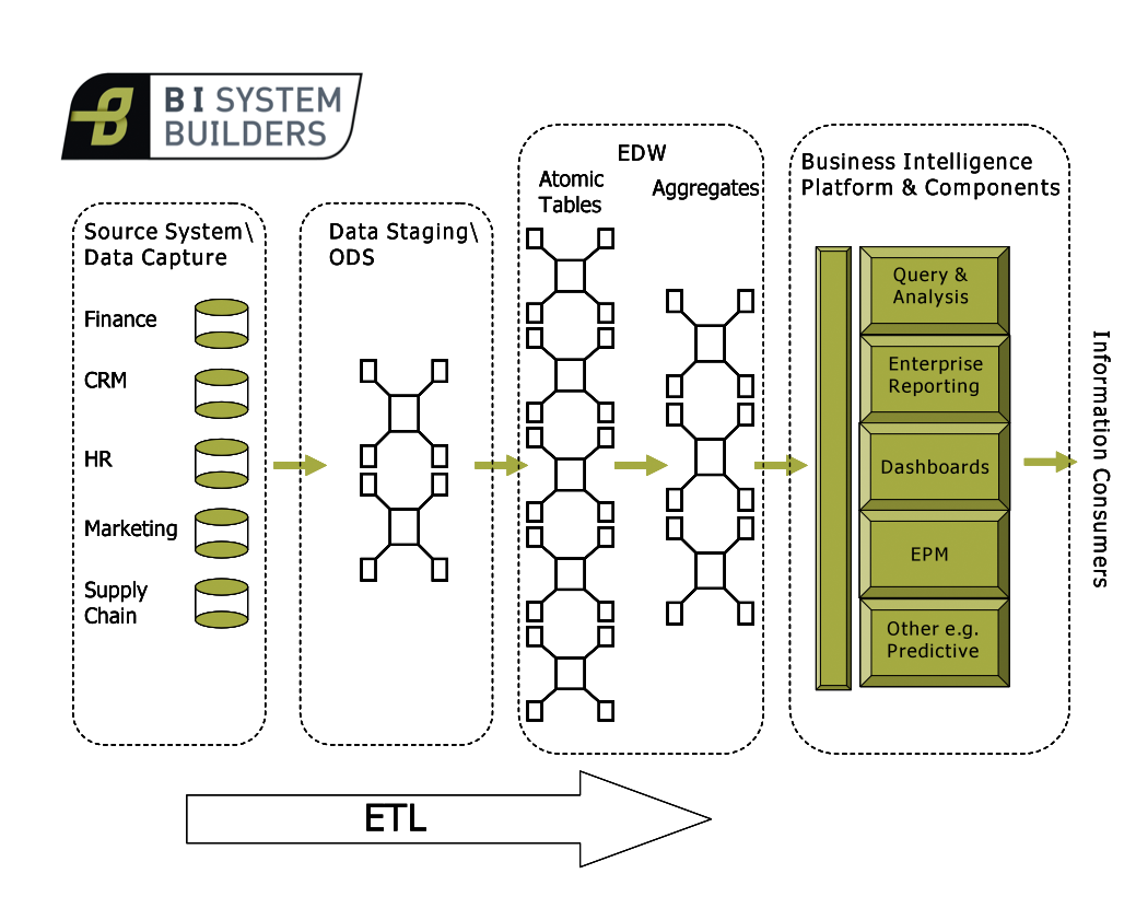
In the previous article we gave an introduction to the End to End BI Philosophy and introduced the various layers that comprise the Business Intelligence Data Warehouse (BIDW). In this article we will focus on getting your End to End BI environment ready by making consideration of sizing and hardware with some reference to software. This article assumes that you are a Business Intelligence Consultant or Architect with design authority or a BI Programme Manager or Business Owner wanting to quickly gain insight into Business Intelligence. If you are technically orientated, your decision making will benefit significantly if you collaborate with an Infrastructure Architect – so go make contact with one in your organisation.
You should plan to size and have hardware procured for five exclusive environments. These are a sandbox, a development environment, a system test environment, and pre-production and production environments. Let’s take a brief look at the nature of these environments.

The sandbox is your playground; it’s a place where you can experiment and learn with zero risk of compromising a deployment on a box used to maintain real content. You can install and configure software, write code and make and break the environment. During my time working for BusinessObjects many software engineers preferred to use VMware for their sandbox. They would install and configure the BI environment and then clone it. Any system corruption – no problem, just blow out the corrupt environment, clone your clean environment again and your back in business. Ensure that the sandbox has sufficient specification to support the minimum requirement of the platforms you intend to install.
The other four environments are where you will manage the lifecycle of your Business Intelligence content. Your development and system test environments are a cut down version of your pre-production environment. Development and system test should run the same software versions and patches as the pre-production and production environments. However the CPU and RAM is usually considerably lower.
The development environment is the place for authorised developers to develop and unit test their code and content. It is not a place for so called ‘ghost’ developers to experiment. Ghost developers are persons that gain access to a development environment with a view to ‘experimenting’ and learning how things work. They will do this anonymously using a generic logon, backdoor or someone else’s password! If you’re a ghost developer, and you know if you are, go play on the sandbox and don’t risk compromising another developer’s hard work on the development environment. At this point you will benefit if you have version control software in place.
After unit testing content on the development environment it is promoted to the system test environment. This is the first time that the testing team will have the opportunity to test the code. To test effectively the system test environment must be stable. Any content identified with defects is passed back to development to be fixed. When content passes testing it is promoted to the pre-production environment. In pre-production we expect high volumes of industrial strength data to be available for the first time. This data may need to be encrypted/ anonymised depending on your industry. It is the opportunity for the content, solution and system to be pressure, stressed, volume tested (PSV) before being unleashed on the production environment. It is a useful place for DBAs to monitor query execution plans and performance tune
Your production environment should mirror your pre-production environment and be secure. By passing content on pre-production testing you are saying that the code is fit to go through the Change Advisory Board (CAB) and move to production. Testing on pre-production is only truly legitimate if the pre-production environment is exactly the same as your production environment.
For brevity the remainder of this article will now focus on the pre-production environment but the concepts can be applied successfully across all four environments. Taking the pre-production environment as our worked example we will need to consider the staging layer, the data mart layer, the ETL system, the Business Intelligence Platform, the RDBMS, hardware and software. This means that there are implications for budget, procurement timelines, licensing, disk space and performance. You may also need to consider contractural terms with third party suppliers of source data and any outsourcing organisations that manage your source systems. If your organisation utilises an ODS or BCNF entity tables you will also need to make other additional considerations. You must now make sizing estimates that will allow you to make informed decisions.
Our first consideration is the BIDW layer known as the staging area as this is where we will (usually) initially land the data. Let’s first of all consider the staging tables. This is the place that you will bring your data in to from outside the BIDW, it’s a kind of landing area. Remember that your sources for Business Intelligence may be wide ranging and include applications such as mainframe legacy systems and an ODS. Your historic load will probably comprise very large data volumes. You will need additional storage space if you need to store the data in flat files etc. before loading to staging. This can happen because of licensing, operating and contractual limitations.
There are three things to consider regarding the architecture and sizing of your staging area. These are the data volumes and nature of your transient staging area, your persistent staging area, and any data archiving area. Your transient data is that data made available to the ETL system for transform and load. You will not want to lose your transient data because you may need to reference it at some point in the future. However, for ETL performance reasons you will not want to hold unnecessarily large volumes of transient data so you will move the data off to your persistent area once the transforms are successful. You must make two decisions. The first is for how long you need to hold your transient data and the second is for how long to hold your persistent data. Let’s say that for legal and audit reasons you decide to persist your staging data for five years. At the end of the period you will need to delete or archive the expired data. To make these decisions you need guidance and remit from senior stakeholders.
It’s time to start making some calculations. Here’s an example thought process. One column field of type integer will equal four bytes. Now let’s say that my staging table has sixty columns that are all of type integer, that’s sixty multiplied by four equals 240 bytes of data per single row. Now let’s say that the source system serves up 60,000 rows of data per night. That’s 60,000 * 240 =14400000 bytes. Ok and let’s say now that I’ll hold my transient data for seven days, that’s 14400000 * 7 = 100800000 bytes of data. Let’s convert that to GBs. 100800000/1024/1024/1024= 0.093877 GB. Let’s say that I have 50 staging tables of similar size loaded every night. That’s equal to 0.093877 * 50 = 4.69GB. Not a lot of space by today’s standards. Now let’s calculate for persisting. That’s 4.69 * 52 (weeks) * 5 (years) = 1219.4 GB or a 1.2 Terabytes of data. We have just calculated your incremental load data for the next five years. You will probably also want to load the historic data held in your source systems. So you must repeat the calculations for the number of years back data (historic) that you want to make available to business users.
So now I have an idea of what disk space I need to procure for staging. Here your Infrastructure Architect can advise on the standard for storing data on a SAN etc. Where possible you should be working within the mandate and standards laid down by the Enterprise Architect.
There are always more details to consider around these areas but the things we have discussed form the backbone of what you will need to think about. There isn’t ‘one size fits all’ but there are frameworks and patterns which repeat themselves again and again. Your considerations now are the procurement, licensing, and installation of any additional/ new RDMS platform and the procurement of any additional hardware to make the staging area performant. In the ideal world these would already be specified in the Solution Architecture, but the reality is that BI Solution Architecture is often overlooked.
The next article in this series will consider your pre-production data marts.


You must be logged in to post a comment.